Monthly Archives: May 2017
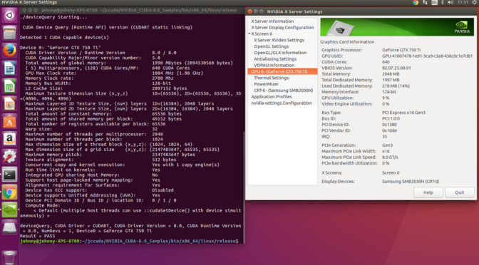
Nvidia CUDA Toolkit Installation (Ubuntu 16.04 LTS) – Notes
(Keeping notes here for ease of future references…)
NumPy Exercise – Argsort and Fancy Indexing
This post summarises my solution to this NumPy Fancy Indexing Exercise (Challenge 3) – originated from scipy-lectures.org
The Problem
Generate a 10 x 3 array of random numbers (in range [0,1]). For each row, pick the number closest to 0.5.
- Use
absandargsortto find the column j closest for each row. - Use fancy indexing to extract the numbers. (Hint:
a[i,j]– the arrayimust contain the row numbers corresponding to stuff inj.)
The Solution
First version code to illustrate how things work:
Now we know how things work, let’s compact the solution (optional).
Major Learning Summary
- Fancy Indexing –
a[rows, cols]ora[[1, 2, 3, 4], [2, 1, 0, 1]] - Sorting –
sort,argsort,argmin/argmax.
NumPy Array Broadcasting: Combine 1D arrays into 2D
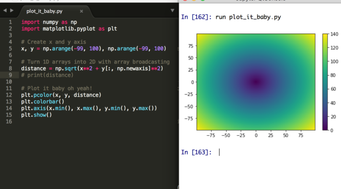
This NumPy Array Broadcasting example is inspired by this SciPy Lecture Chapter on Array Broadcasting.
Code:
Note the use of y[:, np.newaxis].
Note also that this example might be made much simplier with np.ogrid and np.mgrid. (See the SciPy-Lectures chapter on broadcasting)
IPython Jupyter Notebook Trick – Auto Module Reload and Inline Chart Plotting
Two really handy IPython Jupyter Notebook Tricks – Auto Module Reload and Inline Chart Plotting.
Auto Module Reload
Say in our main script we import an external module (that we own). By deafult if we’ve edited that module, it is not automatically reloaded (and therefore won’t take effect in the main script). To enable rapid iteration, it would be very handy to add this IPython magic command at the top – so whenever we’ve updated our module, it’s auto-reloaded in our main script.
Inline Chart Plotting
Another very handy magic command is inline chart plotting (via matplotlib). By default if we do a plot in Jupyter Notebook, a new window will pop up with the chart. If we include the following IPython magic command at the top, our chart may get rendered directly inline within the Jupyter Notebook. (Note that qtconsole by default do the plot inline so we won’t need to worry about that there. Note also that Jupyter Console is text based only and a chart can only be plotted in a new window – i.e. no inline).
Happy rapid iteration!
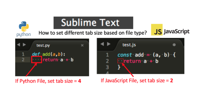
Sublime Text 3 – How to set different tab size based on file type?
Recently I’ve been switching back-and-forth developing in multiple languages, in particular, Python (for backend and data science stuff) and JavaScript (for front-end web demos and ReactJS stuff). As I use Sublime Text 3 to do the code editing, I very often find myself in a situation where I had to manually change the tab size to 4 spaces when coding in Python, and 2 spaces when coding in JavaScript. The manual process eventually got quite painful and tedious so I decided to find out if Sublime Text 3 is clever enough to automatically set the desirable tab sizes based on the file type?
Fortunately the answer is yes – this post documents how (once you know how it only takes less than a minute to setup – Read on!)
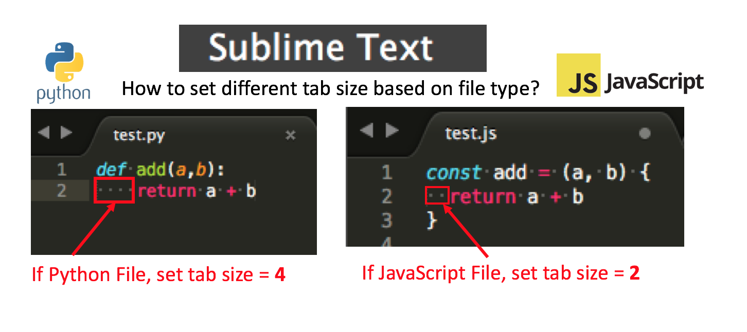
What we want to Achieve
- If we have a Python file, Sublime Text auto set tab size to 4.
- If we have a JavaScript file, Sublime Text auto set tab size to 2.
(and some other desirable tab sizes for other languages – concept is the same).
The Solution
Follow the step-by-step guide – should take about a minute.
Step 1
First, make sure the Python file is opened in editor and active.
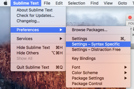
On Mac: Sublime Text -> Preferences -> Settings - Syntax Specific.
(On Windows and Linux I presume it would be something similar)
Step 2
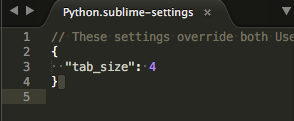
A blank Python.sublime-settings file will open. Simply copy and paste this JASON text to it:
Save and close the file.
Step 3
Repeat Step 1, but this time do it for the JavaScript file.
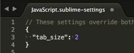
A blank JavaScript.sublime-settings file will open. Simply copy and paste this JASON text to it:
Save and close the file.
Finished!
Now, whenever a Python file is opened, tab size will be set to 4 automatically. And whenever a JavaScript file is opened, tab size will be set to 2 automatically. (Try this out for other languages as you need).
Reference: This Stackoverflow forum
Python NumPy Advance Element Selection Trick – Slice and Jump
TL;DR
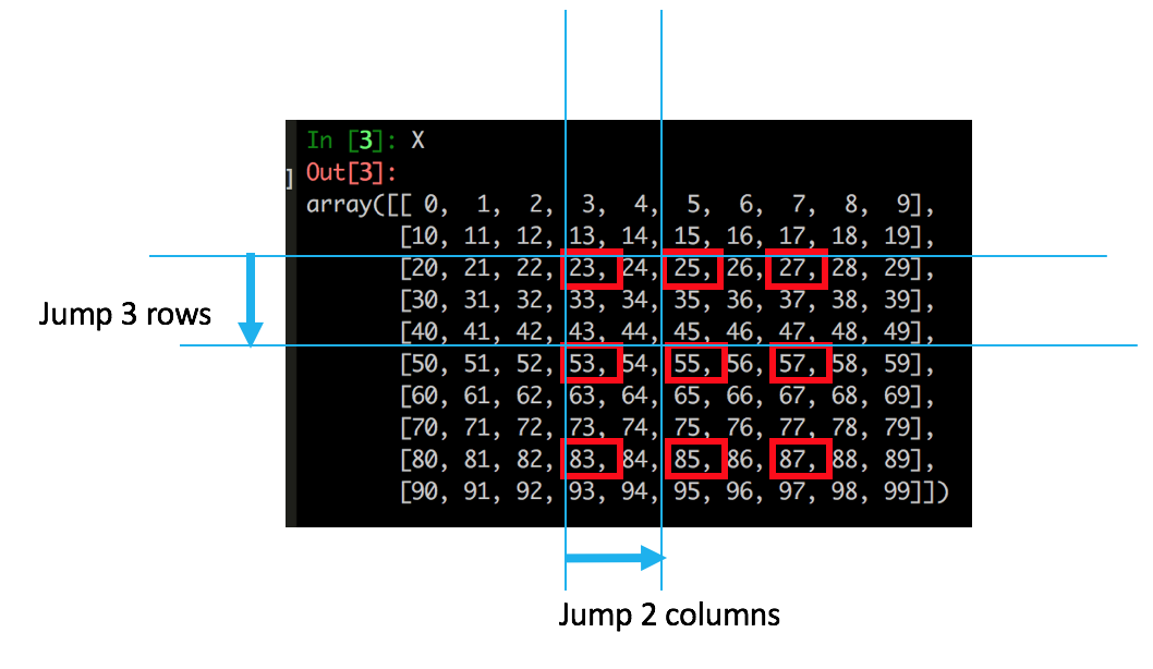
This visual example will show you how to a neatly select elements in a NumPy Matrix (2 dimensional array) in a pretty entertaining way (I promise).
(Caution: this is a NumPy array specific example with the aim of illustrating the a use case of “double colons” :: for jumping of elements in multiple axes. This example does not cover native Python data structures like List).
One concrete example to rule them all…
Say we have a NumPy matrix that looks like this:
    In [1]: import numpy as np

    In [2]: X = np.arange(100).reshape(10,10)

    In [3]: X
    Out[3]:
    array([[ 0,  1,  2,  3,  4,  5,  6,  7,  8,  9],
           [10, 11, 12, 13, 14, 15, 16, 17, 18, 19],
           [20, 21, 22, 23, 24, 25, 26, 27, 28, 29],
           [30, 31, 32, 33, 34, 35, 36, 37, 38, 39],
           [40, 41, 42, 43, 44, 45, 46, 47, 48, 49],
           [50, 51, 52, 53, 54, 55, 56, 57, 58, 59],
           [60, 61, 62, 63, 64, 65, 66, 67, 68, 69],
           [70, 71, 72, 73, 74, 75, 76, 77, 78, 79],
           [80, 81, 82, 83, 84, 85, 86, 87, 88, 89],
           [90, 91, 92, 93, 94, 95, 96, 97, 98, 99]])
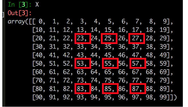
Say for some reason, your boss wants you to select the following elements:
“But How???”… Read on! (We can do this in a 2-step approach)
Step 1 – Obtain subset
Specify the “start index” and “end index” in both row-wise and column-wise directions.
In code:
    In [5]: X2 = X[2:9,3:8]

    In [6]: X2
    Out[6]:
    array([[23, 24, 25, 26, 27],
           [33, 34, 35, 36, 37],
           [43, 44, 45, 46, 47],
           [53, 54, 55, 56, 57],
           [63, 64, 65, 66, 67],
           [73, 74, 75, 76, 77],
           [83, 84, 85, 86, 87]])
Notice now we’ve just obtained our subset, with the use of simple start and end indexing technique. Next up, how to do that “jumping”… (read on!)
Step 2 – Select elements (with the “jump step” argument)
We can now specify the “jump steps” in both row-wise and column-wise directions (to select elements in a “jumping” way) like this:
In code (note the double colons):
    In [7]: X3 = X2[::3, ::2]

    In [8]: X3
    Out[8]:
    array([[23, 25, 27],
           [53, 55, 57],
           [83, 85, 87]])
We have just selected all the elements as required! :)
Consolidate Step 1 (start and end) and Step 2 (“jumping”)
Now we know the concept, we can easily combine step 1 and step 2 into one consolidated step – for compactness:
    In [9]: X4 = X[2:9,3:8][::3,::2]

        In [10]: X4
        Out[10]:
        array([[23, 25, 27],
               [53, 55, 57],
               [83, 85, 87]])
Done!
(I’ve also posted this trick in this Stackoverflow forum)
