Recently I learnt about creating boxplots in R during a Udacity course Data Analysis with R.

Starting off with a sample Pseudo-Facebook CSV Dataset, the aim was to visualize friends-count distribution by gender, using tools such as the R boxplot. The boxplots will enable us to answer questions such as what is the typical distribution profile by gender?, which gender in general have more friend initiations?, are there any improvement opportunities?

There was one major learning relating to the use of applying limits when generating these boxplots, namely the coord_cartesian() method, and the scale_y_continuous() method. These two methods are similar but have very important subtle difference that must not be ignored. I gained this realization from this Udacity Forum.

High level comparison of the two limiting methods

I wish to highlight this very important difference now:

• the coord_cartesian() method creates boxplots first, then zoom-in to the boxplot graphics. (No data points are removed from the boxplot creations).

• the scale_y_continuous() method removes data points first, then creates boxplots graphics (Some data points may get removed from the boxplot creations)

Illustration

The first step is to read the Pseudo-Facebook CSV Dataset into a data object via the RStudio.

pf <- read.csv('pseudo_facebook.tsv', sep = '\t')

To create the basic boxplot, we need to load the ggplot2 package and use the qplot utility.

library(ggplot2)

qplot(x = gender, 
      y = friend_count,
      data = subset(pf, !is.na(gender)), 
      geom = 'boxplot')

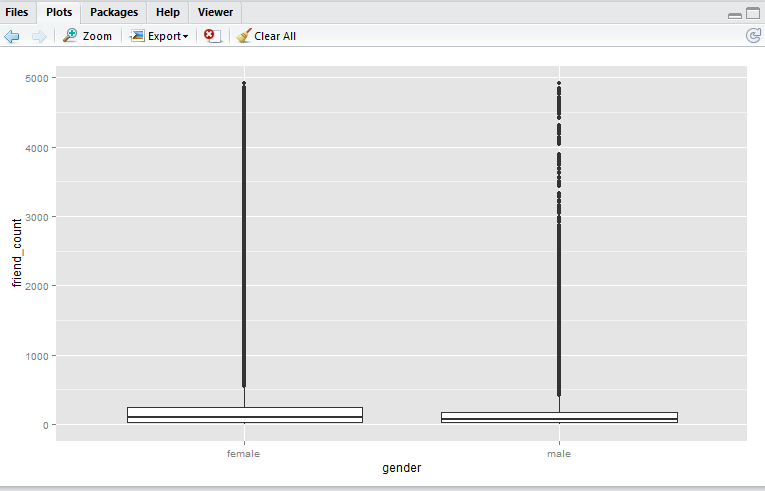
Here we have a boxplot for female, and a boxplot for male. Note that both profiles are fairly long-tail (small distribution of users with abnormaly high friend_count). Now, say we would like to focus on the observations with closer to the box. e.g. friend_count no more than 300.

Here, I would like to show you that coord_cartesian() method will simply zoom-in without altering the boxplots, whereas and the scale_y_continuous() will alter the boxplots completely (as a result of removing data points first, then generate boxplots). Either methods are valid – it depends on whether you wish to keep the (potential) anomaly data in the analysis.

In the following example I shall use 0 as the lower limit, and 300 as the upper limit.

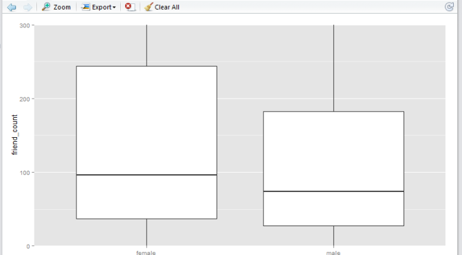
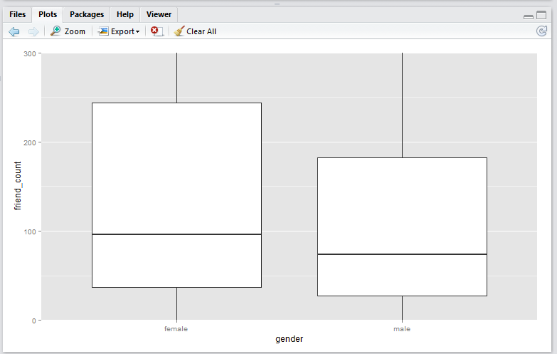
coord_cartesian() method

Script:

qplot(x = gender, 
      y = friend_count,
      data = subset(pf, !is.na(gender)), 
      geom = 'boxplot') +
  coord_cartesian(ylim = c(0, 300))

Output:

scale_y_continuous() method

Script:

qplot(x = gender, 
      y = friend_count,
      data = subset(pf, !is.na(gender)), 
      geom = 'boxplot') +
  scale_y_continuous(limits = c(0, 300))

Output:

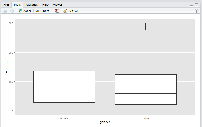
Note that running this script will result in a warning message that looks like this:

Warning message:
Removed 16033 rows containing non-finite values (stat_boxplot). 

Observation

• Note that the coord_cartesian() method produces a boxplot that is exactly the same as the original boxplot. This is becuase the boxplot is created using the entire set of data points, just like the original. This plot is useful if you wish to analyse all the data points and just want to zoom-in to the data.

• Note that the scale_y_continuous() method shift the box (25th to 75th percentile) downwards. This is because the all the datapoints above 300 are removed before the boxplot is generated. This plot is useful if you wish to analyse only the data within the limiting range.

Conclusion

In this article I have presented two boxplot methods, namely the coord_cartesian() method, and the scale_y_continuous(). The coord_cartesian() method is suitable if you wish to analyse all of the incoming data before creating the boxplots. The scale_y_continuous() method is suitable if you would like to drop all the data beyond the limiting range prior creating the boxplots.

---

Discussion

Do you have any interesting experiences relating to creating boxplots with R? Feel free to leave a comment!